Introduction

Two open source Modelica front-ends are actually available OpenModelica and JModelica. We will review these two solutions and present their respective advantages and drawbacks.

OpenModelica provides a GUI based on the Qt4 framework that aims to offer a standalone Modelica environement similar to Dymola, i.e. a model editor, a schema (annotation) editor, an interface to set up the simultation and an interface to plot results. Actually (version 1.9) the schema editor is able to draw annotations, but it is not really usable for edition. In comparison the Scicos editor looks more finished. Despite a standalone environement has some advantages, the editor and the plot functions can be replaced by other software. For example the editor and the simultation setup can be performed within the Eclipse Framework and the ploting within the Python environment.

An Example of Modelica Model

We will use as example a model of a simple rectifier with a transformer:

model FullWaveBridgeWithTransformer
  Modelica.Electrical.Analog.Sources.SineVoltage ac_line(V = 230, freqHz = 50);
  Modelica.Electrical.Analog.Basic.Capacitor capacitor(C = 50e-6);
  Modelica.Electrical.Analog.Basic.Ground ground;
  Modelica.Electrical.Analog.Ideal.IdealDiode diode(Vknee = 0.5);
  Modelica.Electrical.Analog.Basic.Resistor load_resistor(R = 1e3);
  Modelica.Electrical.Analog.Ideal.IdealTransformer transformer(n = 10, Lm1 = 1);
equation
  connect(ac_line.p,transformer.p1);
  connect(ac_line.n,transformer.n1);
  connect(ac_line.n,ground.p);
  connect(transformer.p2,diode.p);
  connect(transformer.n2,ground.p);
  connect(diode.n,capacitor.p);
  connect(diode.n,load_resistor.p);
  connect(capacitor.n,ground.p);
  connect(load_resistor.n,ground.p);
end FullWaveBridgeWithTransformer;

JModelica

JModelica is fully integrated within Python through several modules. The JModelica installation provides in the jmodelica-1.9/bin directory two scripts, jm_python.sh and jm_ipython.sh to wrap the Python interpreter and the IPython interactive interpreter, respectively. Theses scripts initialise some environment variables before to run the interpreter.

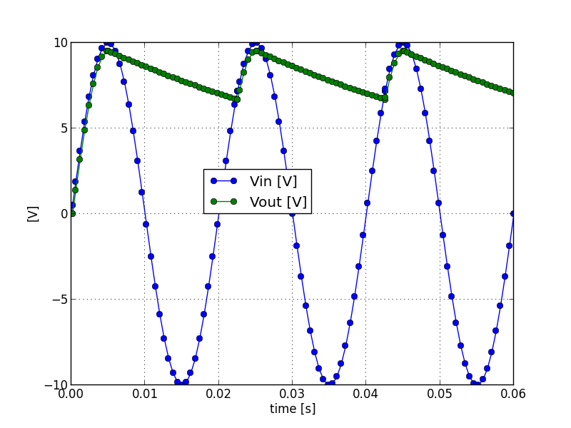
The following Python script shows how to genrate a FMU module, simulate it, retrieve the results and plot them using the Matplotlib module:

from pymodelica import compile_fmu
from pyfmi import load_fmu

import pylab as pylab

class_name = 'SimpleRectifierWithTransformer'
model_path = class_name + '.mo'

# Compile and load the FMU
fmu_name = compile_fmu(class_name, model_path)
fmu = load_fmu(fmu_name)

# Set model constants and simulate
fmu.set('ac_line.V', 100)
options = {
    'ncp':100, # number of communication points
    }
result = fmu.simulate(final_time=3/50., options=options)

# Get variable values
t = result['time']
vin = result['transformer.v2']
vload = result['load_resistor.v']

# Plot
pylab.grid()
pylab.plot(t, vin, 'o-', t, vload, 'o-')
pylab.xlabel('time [s]')
pylab.ylabel('[V]')
pylab.legend(('Vin [V]', 'Vout [V]'), loc=(.3,.5))
pylab.show()

OpenModelica

There is several ways to simulate a model with OpenModelica. All these ways use the OpenModelica omc compiler to generate a stand-alone simulation executable. The compiler can be called from the shell or via a Corba interface. The Corba interface is used by the OMEdit GUI, the OpenModelica shell omshell and the OMPython Python module.

The omc compiler can be steered with a mos script file that contain instructions, for example to load the model, simulate the model and plot results.

loadModel(Modelica);
loadFile("SimpleRectifierWithTransformer.mo");
simulate(SimpleRectifierWithTransformer, startTime=.0, stopTime=3/50., numberOfIntervals=100);
plot({transformer.v2, load_resistor.v});

To run this mos script file, copy-paste this command in the shell:

omc sim_SimpleRectifierWithTransformer.mos

This command will generate the C source files of the simulation executable, a Makefile to compile the executable, the executable, two XML files and a mat file that contains the results.

We can run the simulation and override some parameters like this:

SimpleRectifierWithTransformer -override ac_line.V=100

And finally plot the result using the OMPlot command:

OMPlot --filename=SimpleRectifierWithTransformer_res.mat ac_line.v transformer.v2 load_resistor.v

This process can also be performed from Python using a CORBA interface provided by the OMPython:

import OMPython
for command in (
  'loadModel(Modelica)',
  'loadFile("SimpleRectifierWithTransformer.mo")',
  'simulate(SimpleRectifierWithTransformer, startTime=0.0, stopTime=3/50., numberOfIntervals=100)',
  'plot({transformer.v2, load_resistor.v})' ,
  ):
  answer = OMPython.execute(command)
  print "\nResult:\n%s" % answer

The simulation results are written in a mat file which is equivalent to a Dymola file and similar to a Matlab file. The DyMat package provides some modules to read and process the result files from Dymola and OpenModelica with python. It also provides a script to export the mat file to other format like HDF5 for example.

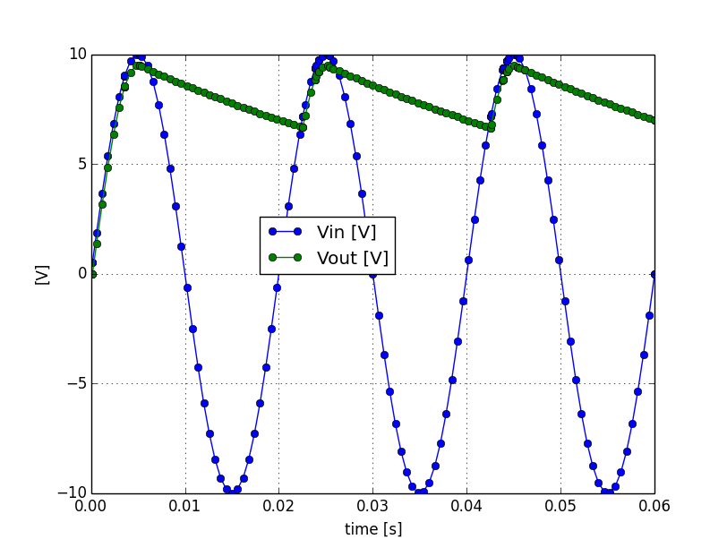
This Python script shows how to use it and plot result using Matplotlib:

import pylab
import DyMat

# Get variable values
mat = DyMat.DyMatFile("SimpleRectifierWithTransformer_res.mat")
t = mat.abscissa('transformer.v2')[0]
vin = mat.data('transformer.v2')
vload = mat.data('load_resistor.v')

# Plot
pylab.grid()
pylab.plot(t, vin, 'o-', t, vload, 'o-')
pylab.xlabel('time [s]')
pylab.ylabel('[V]')
pylab.legend(('Vin [V]', 'Vout [V]'), loc=(.3,.5))
pylab.show()