Introduction

SPICE (Simulation Program with Integrated Circuit Emphasis) was developed at the Electronics Research Laboratory of the University of California, Berkeley in 1973 by Laurence Nagel with direction from his research advisor, Prof. Donald Pederson. Then Spice emerged as an industrial standard through its descendant and is still the reference 40 years later.

The last version released at Berkeley on 1996 is spice3f5.

The technical report No. UCB/ERL M520 written by Nagel gives an interesting description of the algorithms involved in Spice. I recommend to read the part 2 and 3 that explain the equation formulation. The next parts describes the numerical analysis.

A basic example to introduce circuit modelisation in Spice

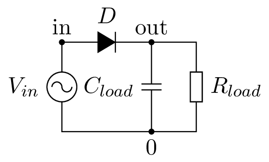
Circuits are modelled by a simple language, for example a simple rectifier could be modelled as follow:

.. code-block:: spice

  .title Simple Rectifier
  .include 1N4148.lib
  .param line_peak_voltage=230V
  .param freq=50Hz
  * A comment before to start the net list:
  Vinput in 0 DC 0V SIN(0V {line_peak_voltage} {freq})
  xD in out 1N4148
  Cload out 0 100uF
  Rload out 0 1k
  .end

This model is made of a sinusoidal source, a rectifier diode, a filter capacitor and a resistor load.

The lines starting by a dot are special directives that indicate here the title of the circuit, a file inclusion and two parameter definitions. The other lines define the element in the circuit, the so called net list.

Each element in the circuit is specified by an element line that contains:

• the element name,
• the circuit nodes to which the element is connected,
• and the values of the parameters that determine the electrical characteristics of the element.

An element name starts with a letter that define the type of device, for example C for capacitor and R for resistor. This letter is suffixed by an user name to identify uniquely the element.

The model of the 1N4148 diode is provided in a separate file. Usually manufacturers provide Spice models for their devices on their web sites. This file can be downloaded here and it contains the definition of a sub-circuit made of a diode and a large resistance in parallel to improve modeling in the reverse mode of operation:

.. code-block:: spice

  .subckt 1N4148 1 2
  R1 1 2 5.827E+9
  D1 1 2 1N4148
  .model 1N4148 D
  + IS = 4.352E-9
  + N = 1.906
  + BV = 110
  + IBV = 0.0001
  + RS = 0.6458
  + CJO = 7.048E-13
  + VJ = 0.869
  + M = 0.03
  + FC = 0.5
  + TT = 3.48E-9
  .ends

A line starting with a + indicates the previous line continue here. The .model directive defines a device model called 1N4148 for the diode which is based on the diode Spice model (identified by D) and parametrised by the following lines.

The chapter 2 of the ngspice manual gives a complete overview of the circuit description and the following chapters describes the available device models.

Spice and its derivatives

Since the source code of Spice was open, many derivatives forked from the original source code of Berkeley, some are commercial like PSpice of Cadence and LTspice of Linear Technology, or open source like ngspice and gnucap.

Ngspice (New Generation Spice) is the open source successor of spice3f5 featuring a mixed-level and mixed-signal circuit simulator. It is based on an updated version of spice3f5 and enhanced with XSpice (mixed signal), Cider1b1 and GENIUS TCAD (mixed level). Ngspice is still maintained by a group of maintainers and the version 25 was released on January 3rd, 2013.

Gnucap (GNU Circuit Analysis Package) was an attempt to rewrite Spice from scratch by Albert Davis in 1993, but the last version was delivered in 2006 and now the project is no longer active (excepted some commits in the Git repository in 2013). The thesis of Albert Davis entitled "Implicit Mixed-Mode Simulation of VLSI Circuits" contains information on circuit computation and simulation.

A rewrite of spice3f5 from scratch is justified since it was developed as a research project rather than an industrial software. The code is mostly undocumented and relatively impenetrable, thus it will probably not evolved any more.

Non Spice compatible Simulator

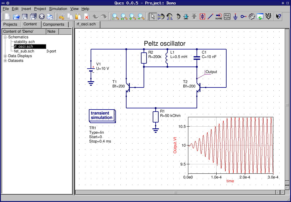
Qucs (Quite Universal Circuit Simulator) is a "non Spice compatible" circuit simulator founded by Michael Margraf in 2003 (?), where circuits are modelled through a graphic user interface and later serialised to an XML format. The Qucs tool chain features a simulator and a graphic user interface for schematic capture, simulation setup and to display results.

For simulation of Spice netlists within Qucs see this tutorial.

The technical document contains information on circuit computation and simulation within Qucs (see also this link for more references).

Qucs GUI was originally developed using the Qt3 framework and a port to Qt4 was started some years ago. Unfortunatelly the project was sleeping these last years and the original founder is not longer active on this project. I think it is a mistake to aim to develop a complete toolchain in a non commercial context, since it is too much work for a small team working on the project during its free time. Just the GUI maintenance (Qt4 port) require a lot of work.

Ngspice Compilation

We will now focus on Ngspice since it is the most mature and active descendant of spice3f5.

Usually Ngspice is available as a package in the major Linux distributions. But I recommend to check the compilation options before to use it extensively. For example the Fedora package enables too many experimental codes that have side effects. The recommended way to compile Ngspice is given in the manual and the INSTALLATION file. Ngspice is an example of complex software where we should not enable everything without care.

Ngspice Tool Chain

For historical reason Ngspice features a complete tool chain which is made of:

• a Spice front-end to parse the circuit description,
• some device models,
• a circuit simulator,
• an interactive interpreter to steer a model simulation and analyse results,
• a graphical tool to display results.

Nowadays we can replace the analysis tool by the Python environment and only use the heart of Ngspice for circuit simulation. Thus it would be nice to package the simulator in a C library and steer the circuit and simulation through an API accessible from Python.

The TCL module Tclspice of Ngspice uses partially this approach to embed Spice in TCL. But it is more a hack than a clean approach. Indeed this module uses the interpreter functions to communicate with Ngspice. For example a circuit definition is read using the command source which read the circuit from a C file handle and not from a string buffer. However probe values are accessed through internal C data structures.

We could try a similar approach for Python, but the source code of Ngspice is mostly undocumented and quite impenetrable. Thus by pragmatism we will first use a pipe to connect Ngspice and Python all together.

Ngspice and Python Interplay

We will now test our Ngspice-Python bridge approach using our simple rectifier example.

First we will write a flattened version of the code to the file simple-rectifier.cir:

.title Simple Rectifier
.subckt 1N4148 1 2
R1 1 2 5.827E+9
D1 1 2 1N4148
.model 1N4148 D IS = 4.352E-9 N = 1.906 BV = 110 IBV = 0.0001 RS = 0.6458 CJO = 7.048E-13 VJ = 0.869 M = 0.03 FC = 0.5 TT = 3.48E-9
.ends
Vinput in 0 DC 0V SIN(0V 10V 50Hz)
xD in out 1N4148
Cload out 0 100uF
Rload out 0 1k
*
.options TEMP=25 TNOM=25
.options NOINIT
.options filetype = binary
.tran 0.0001 0.1
.save V(in) V(out)
.end

We have added at the end of the file the .tran directive to indicate we want a transient analysis from t = 0 to 100 ms with a step of 100 us. We also setup some options to indicate we want to simulate the circuit at a temperature of 25° and a binary output.

Now we run this command using pipe and redirection in the shell:

cat simple-rectifier.cir | ngspice -s > output.raw 2> number_of_lines.txt

The output.raw file (standard output) must contain a text header and then binary data:

Circuit: Simple Rectifier

Doing analysis at TEMP = 25.000000 and TNOM = 25.000000

Title: Simple Rectifier
Date: Sun Dec 29 02:55:40  2013
Plotname: Transient Analysis
Flags: real
No. Variables: 3
No. Points: 0
Variables:
No. of Data Columns : 3
        0       time    time
        1       v(in)   voltage
        2       v(out)  voltage
Binary:
...

The number_of_line.txt file (standard error) must contain this line:

@@@ 127 1016

where 1016 is the number of points of the simulation. The output is written during the analysis, thus the number of points is only known afterwards.

The binary data after the line Binary: is the serialisation of an array of dimension (number of lines, number of columns) = (1016, 3) of type double (8 bytes). Depending of the analysis, the values can be real or complex. Complex values are serialised to two doubles and thus count twice.

We can now plot the waveforms using the IPython interactive environment. To do this, we have first to launch the environment using the command ipython --pylab and then copy-past this code in the terminal:

import os
import numpy as np

raw_file = 'output.raw'
number_of_probes = 3
number_of_points = 1016

with open(raw_file, 'r') as f:
    while f.readline() != 'Binary:\n':
        pass
    location= f.tell()

expected_size = location + number_of_probes * number_of_points * np.double().nbytes
assert(os.stat(raw_file).st_size == expected_size)

shape = (number_of_points, number_of_probes)
probes = np.memmap(raw_file, mode='r', offset=location, shape=shape, dtype='d')
probes = probes.transpose()

figure, (axe1, axe2) = subplots(ncols=2)
axe1.plot(probes[0], probes[1], probes[0], probes[2])
axe1.set_xlabel('time [s]')
axe1.set_ylabel('[V]')
axe1.legend(('Vin [V]', 'Vout [V]'), loc=(.3,.5))
axe2.plot(probes[1], probes[2])
axe2.set_xlabel('Vin [V]')
axe2.set_ylabel('Vout [V]')

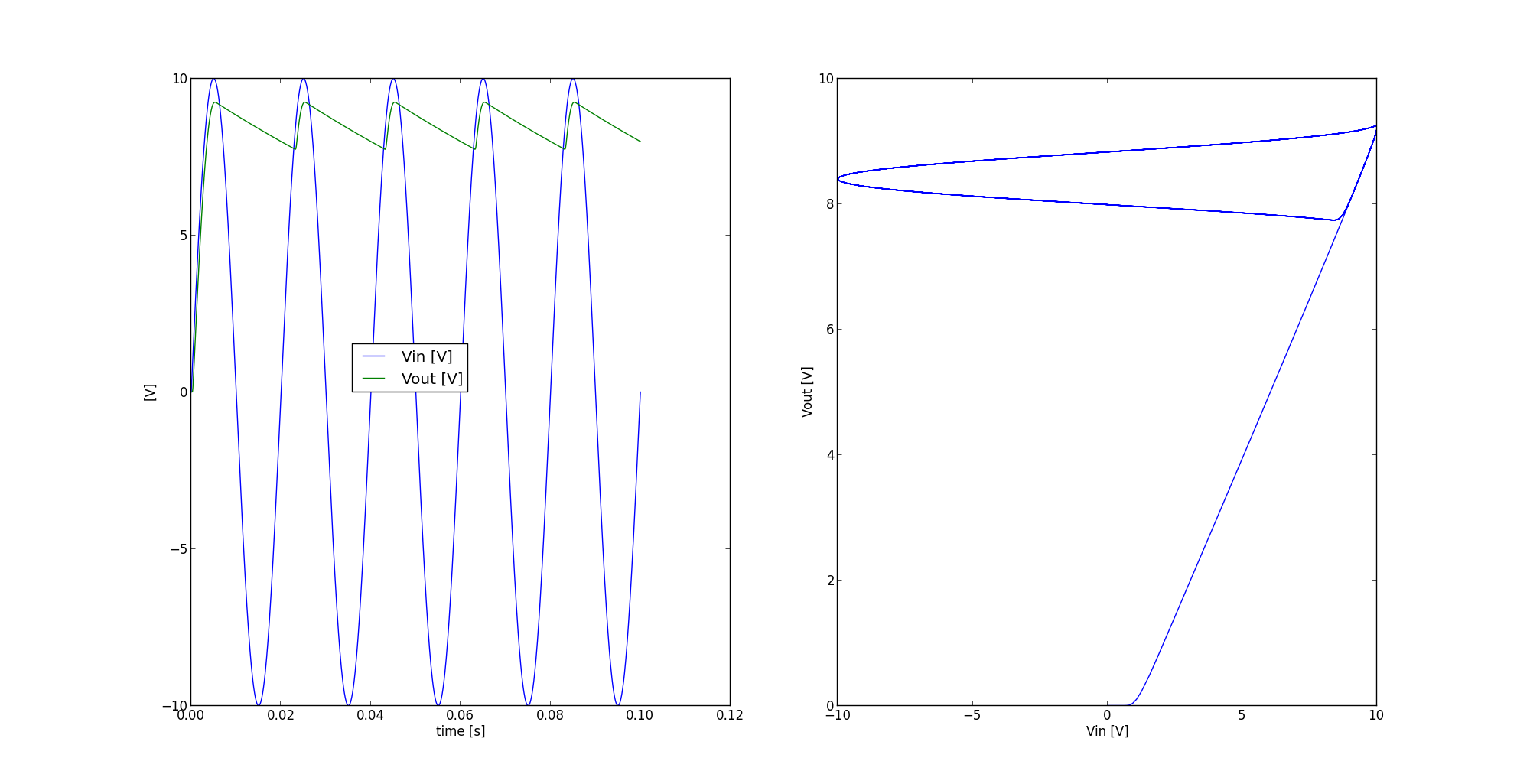
The size of the binary output is tested so as to ensure the output is right.

We have now all the keys to write a more elaborated Python module to interconnect Ngspice with the Python environment.

References

The relevant references on Spice are by date of publication:
- Technical Report No. UCB/ERL M382; SPICE (Simulation Program with Integrated Circuit Emphasis); Nagel, Laurence W. and Pederson, D.O.; April 1973
- Technical Report No. UCB/ERL M520; SPICE2: A Computer Program to Simulate Semiconductor Circuits; Nagel, Laurence W.; 1975
- Technical Report No. UCB/ERL M89/42; Analysis of Performance and Convergence Issues for Circuit Simulation; Quarles, Thomas L.; 1989
- official spice3f5 source code on eecs.berkeley.edu server, the page contains some links on Spice (historical notes).